A benchmark dataset for mapping land-cover in Europe

Prepared and maintained by: Leandro Parente (OpenGeoHub), Martijn Witjes (OpenGeoHub)

Mapping the land-cover (LC) dynamics over the past two decades (2000 to 2020) for Continental Europe is one of the main goals of the Geo-Harmonizer project. To generate annual predictions of land cover, we will use a spatiotemporal machine learning model, able to generalize in space and time, to predict the LC in any part of the European territory over different years. To be successful with this type of approach (spacetime prediction) we should use high quality training samples, collected in different years, and several harmonized raster layers, correlated with the LC in the EU. Here we provide two benchmark datasets, which will be useful for training and evaluating different space time models for LC mapping in the project.

To create the training samples we combined points from CORINE and LUCAS survey, obtained in different years (2000, 2006, 2009, 2012, 2015 and 2018) and distributed throughout the European territory. All the samples had two or more LC classes over the years, and 22% of the points suffered some type of LC change. The LC classes were harmonized and reduced to 32 possibilities:

• Port areas (code 123)
• Airports (code 124)
• Mineral extraction sites (code 131)
• Dump sites (code 132)
• Construction sites (code 133)
• Non-irrigated arable land (code 211)
• Permanently irrigated arable land (code 212)
• Rice fields (code 213)
• Vineyards (code 221)
• Fruit trees and berry plantations (code 222)
• Olive groves (code 223)
• Pastures (code 231)
• Broad-leaved forest (code 311)
• Coniferous forest (code 312)
• Natural grasslands (code 321)
• Moors and heathland (code 322)
• Sclerophyllous vegetation (code 323)
• Transitional woodland-shrub (code 324)
• Beaches, dunes, sands (code 331)
• Bare rocks (code 332)
• Sparsely vegetated areas (code 333)
• Burnt areas (code 334)
• Glaciers and perpetual snow (code 335)
• Inland wetlands (code 411)
• Maritime wetlands (code 421)
• Water courses (code 511)
• Water bodies (code 512)
• Coastal lagoons (code 521)
• Estuaries (code 522)
• Sea and ocean (code 523)

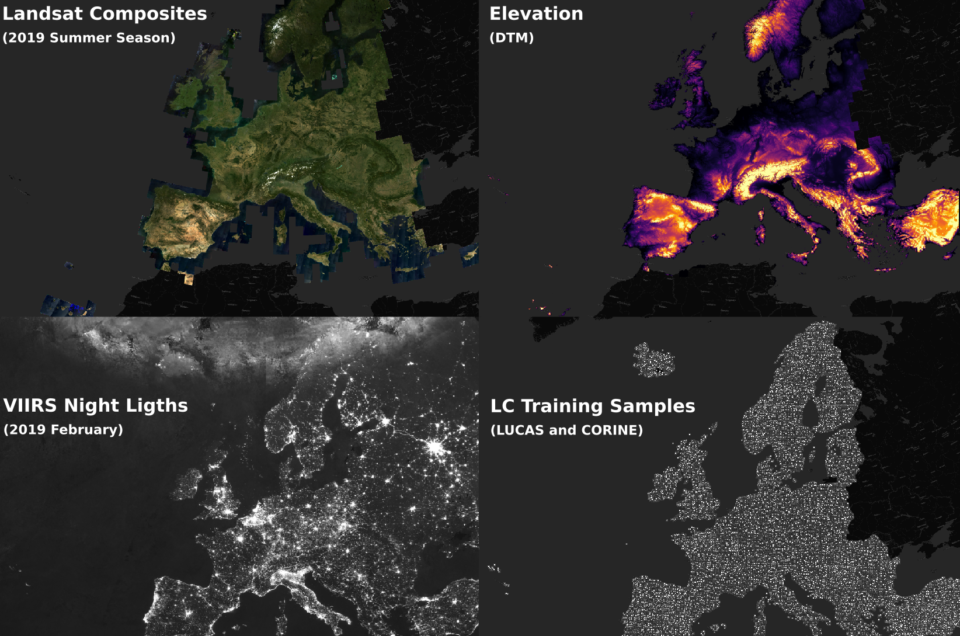
As raster layers we used satellite data, obtained from SUOMI-NPP (VIIRS) and Landsat (TM, ETM+ and OLI), and Digital Terrain Model-DTM data, derived from Ensemble ML estimation. From VIIRS data we extracted the night band (VNP46A1 product), using the best image available in each year (low cloud contamination and high surface coverage), and from DTM we extracted the elevation and slope layers. For Landsat data, we downloaded all the GLAD Analysis Ready Data-ARD available for the EU since 2000, removed all the pixels contaminated by cloud and cloud shadows (Quality Assessment band), and calculated 3 percentiles (25, 50, 75) for each season, on a yearly basis and for all the bands (Blue, Green, Red, NIR, SWIR1, SWIR2 and Thermal). The seasons were defined using the same calendar dates for the whole period:

• Winter: December 2 of previous year until March 20 of current year
• Spring: March 21 until June 24 of current year
• Summer: June 25 until September 12 of current year
• Fall: September 13 until December 1 of current year

Even using the Glad ARD, which combines the 3 Landsat sensors (TM, ETM+ and OLI), and multiple months for each season, the temporal composites presented several nodata gaps (mostly in winter season). To handle with this issue, we implemented a very basic approach to fill the gaps using 1) the long-term median value for each season (winter median of P50 NIR between 2000 and 2020), and for remaining gaps 2) the long-term median for all period (median of P50 NIR between 2000 and 2020). This approach was implemented in python (Jupyter notebook), however we are evaluating other gap filling strategies availables in R (gdalcubes) and in peer-review papers (https://doi.org/10.3390/rs12071192, https://doi.org/10.1016/j.rse.2018.04.042).

Currently we have more than 5.5 millions training samples and 87 raster layers (84 from Landsat, 1 from VIIRS and 2 from DTM) to train and evaluate our spacetime ML-model (contact leandro.Parente@opengeohub.org for more info). These datasets were organized in a EU tiling system, which consists of 7,042 regular tiles with 30 x 30 km, and based on it, we make available 2 pilot tiles (Croatia and Sweden) in Zenodo to test our LC mapping workflow (eumap v0.1.0). For all steps (gap filling, space time overlay and land-cover classification) we created a tutorial to demonstrate how to use these approaches in python.

Image: General workflow describing how are Landsat ARD composites, in combination with other landform and EO covariates, used to produce complete consistent time-series that can be used for land cover classification.

In the next months we will release the EU Landsat temporal composites gap-filled and harmonized with Sentinel-2 data (from 2018), as well as the EU night light layer, and all the functions developed for our LC mapping workflow will be publicly available on eumap. To follow the progress of the project please connect to our Twitter channel.

 337 total views,  2 views today