Prepared and maintained by: Leandro Parente (OpenGeoHub), Ognjen Antonijevic (GiLAB), Tom Hengl (OpenGeoHub), Luka Glusica (GiLAB), Martin Landa (CVUT Prague)
This tutorial explains (a) how to access Geo-harmonizer geospatial layers, (b) how to use them as a database i.e. to query, subset and download, (c) how to visualize data in QGIS or similar. Software requirements:
Connected repository: https://gitlab.com/Geo-harmonizer_inea/spatial-layers
Accessing and viewing data
Raster or gridded data
Geo-harmonizer serves a number of raster or gridded layers, usually prepared as Cloud-Optimized GeoTIFFs at 30 m or coarser resolution.
Vector data
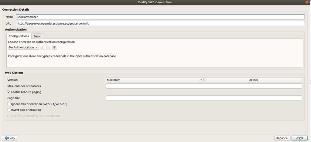
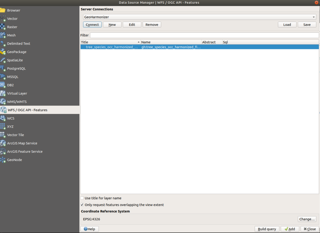
Data can be imported into QGIS in a standard way through WFS service using URL:
https://geoserver.opendatascience.eu/geoserver/wfs
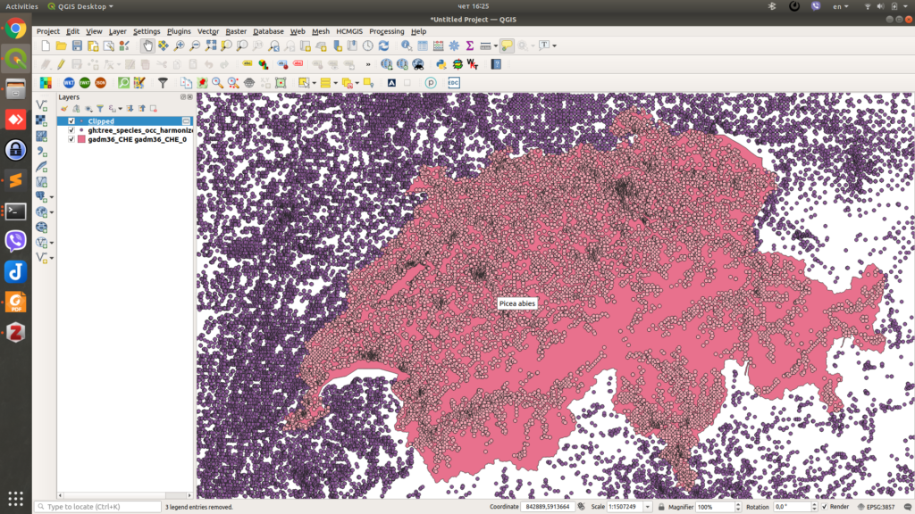
The loading might take some time because the dataset is large, therefore it’s best to first zoom to area or feature of interest (for example Switzerland in the image below)
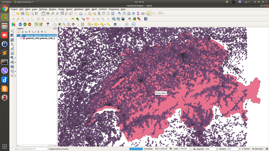
From then on, you can perform all standard operations as with any other vector datasource in QGIS. For example clip data for this country:
It’s also possible to access this data as GeoJSON directly through browser:
There are various options supported for GetFeatures request:
https://docs.geoserver.org/latest/en/user/services/wfs/reference.html#getfeature
And this service can be used directly from GDAL library:
https://gdal.org/drivers/vector/wfs.html
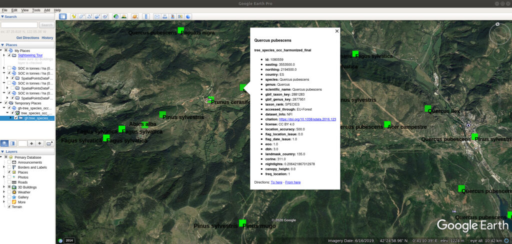
To view vectors in Google Earth, visit the GeoServer page and then select Download -> KML -> Network link. Once you download the KML you need to zoom-in to an area of interest and then the points with labels should be visible directly in Google Earth.
Opening data in QGIS
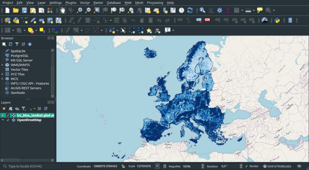
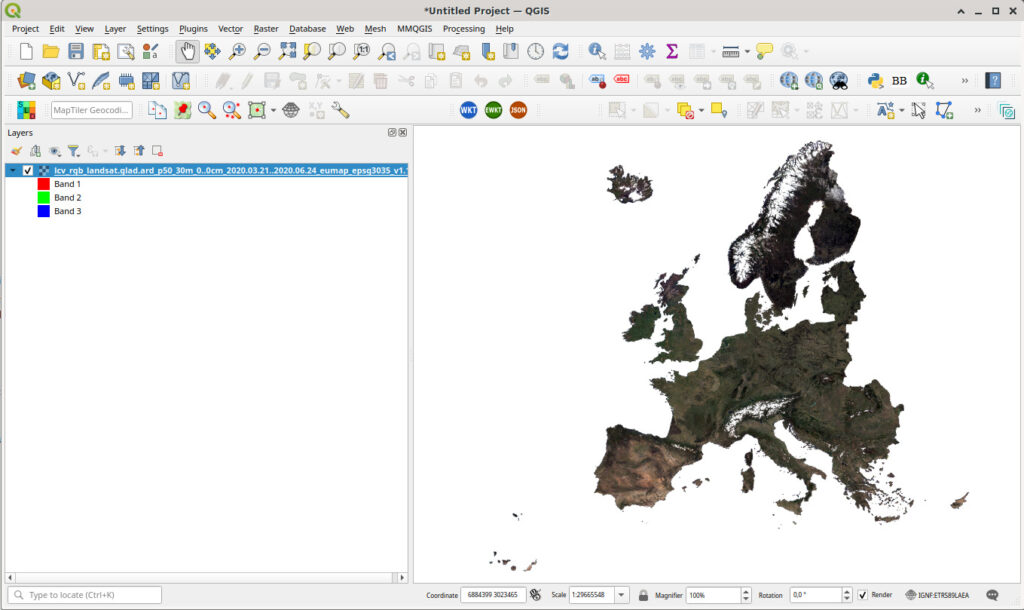
Geo-harmonizer raster layers can be accessed through HTTP service using QGIS (see also the COG tutorial). These are example of layers:
- Quarterly GLAD Landsat RGB composite: http://s3.eu-central-1.wasabisys.com/eumap/lcv/lcv_rgb_landsat.glad.ard_p50_30m_0..0cm_2020.03.21..2020.06.24_eumap_epsg3035_v1.1.tif
- Quarterly GLAD Sentinel-2 L2A RGB composite: http://s3.eu-central-1.wasabisys.com/eumap/lcv/lcv_rgb_sentinel.s2l2a_p50_30m_0..0cm_2020.03.21..2020.06.24_eumap_epsg3035_v1.0.tif
Processing data using GDAL and R
To download data from COG repository best use GDAL utilities either gdal_translate or gdalwarp. This allows you to subset, reproject, translate data without a need to download the complete repository that could be tens of Terabytes in size.
Using GDAL utils on COGs
To demonstrate the usage of GDAL commands we will use a bounding box covering Amsterdam, projected in the ETRS89-extended / LAEA Europe coordinate system (EPSG:3035). A easy way to get this information is using the QGIS bounding box plugin:
- ulx (xmin): 3949019.319534085
- uly (xmax): 3274684.0278522763
- lrx (xmax): 3997655.528969183
- lry (ymin): 3247994.5591947753
The gdal_translate can be used to download data directly from a COG URL. You just need to pass the bounding box information as a -projwin parameter, informing the COG url prefixed by /viscurl/:
| gdal_translate -co COMPRESS=LZW -projwin 3949019.319534085 3274684.0278522763 3997655.528969183 3247994.5591947753 /vsicurl/http://s3.eu-central-1.wasabisys.com/eumap/lcv/lcv_rgb_landsat.glad.ard_p50_30m_0..0cm_2020.03.21..2020.06.24_eumap_epsg3035_v1.1.tif amsterdam.tif |
It’s also possible to reproject on-the-fly the raster output, generating an image in, for example, WGS84 projection (EPSG:4326). First it’s necessary to create a VRT file using gdalbuildvrt command (take careful with the different order for the bounding box coordinates in -te):
| gdalbuildvrt -te 3949019.319534085 3247994.5591947753 3997655.528969183 3274684.0278522763 amsterdam_4326.vrt /vsicurl/http://s3.eu-central-1.wasabisys.com/eumap/lcv/lcv_rgb_landsat.glad.ard_p50_30m_0..0cm_2020.03.21..2020.06.24_eumap_epsg3035_v1.1.tif |
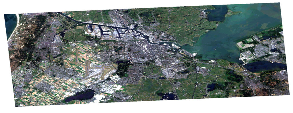
Now just execute a regular gdalwarp informing the desired projection:
| gdalwarp -overwrite -co COMPRESS=LZW -t_srs ‘EPSG:4326’ amsterdam_4326.vrt amsterdam_4326.tif |
The projected result should be like this
Overlaying large set of points with COGs
To query the data for any coordinate/point of EU check this Jupyter notebook tutorial.
Clipping maps to a smaller subarea
To access the Geo-harmonizer datasets through STAC check this Jupyter notebook tutorial.
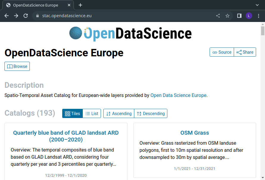
Using the STAC browser
All GeoHarmonizer datasets and their respective metadata are listed in a Spatio-Temporal Asset Catalog (STAC): https://s3.eu-central-1.wasabisys.com/stac/odse/catalog.json.
The data can be browsed through using the STAC Browser hosted as part of the ODSE portal:
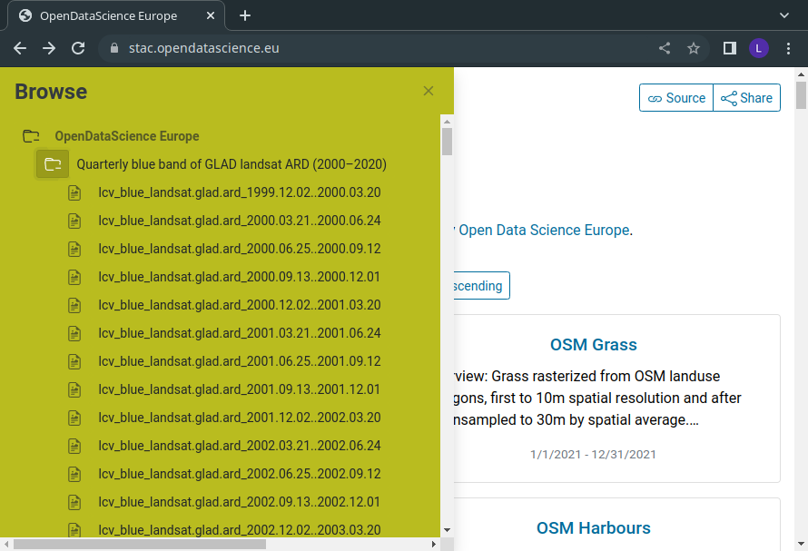
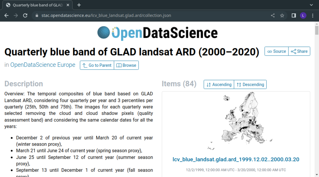
Complete metadata can be accessed using the browser for entire collections:
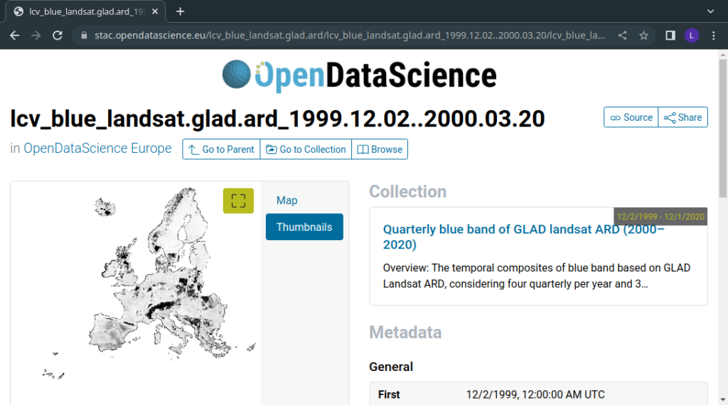
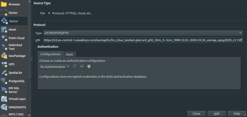
For each asset in a datasets there are file URLs (in this case for a Cloud Optimized GeoTiff) that can be accessed with your GIS software of choice:
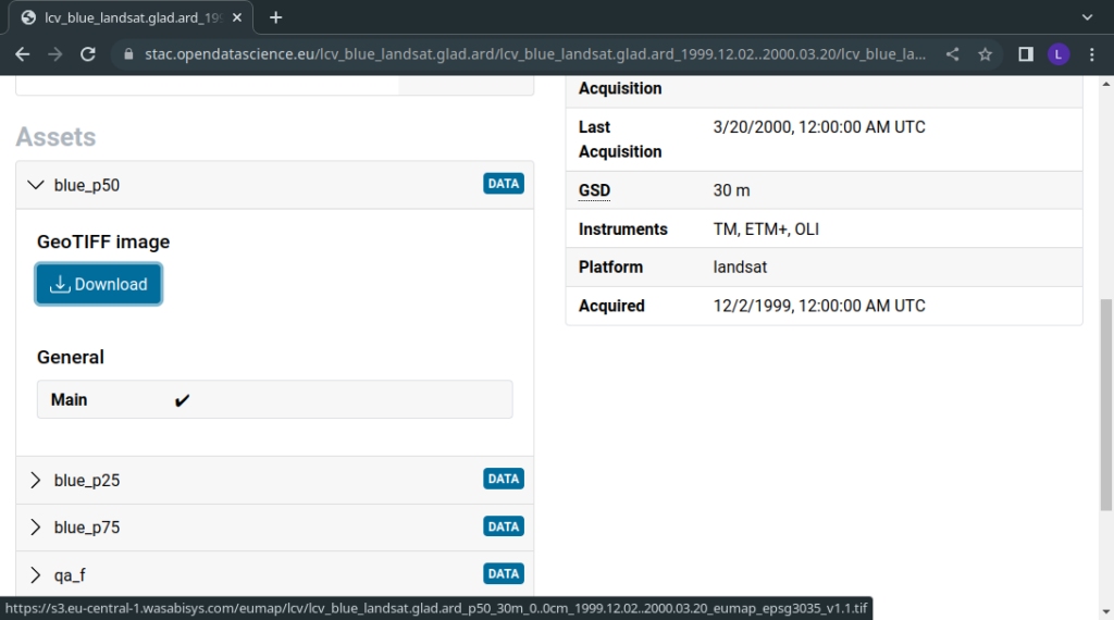
As an example, the image above can be accessed with QGIS by copying the download URL and creating a raster layer with network protocol as the source type: